Understanding Sound from First Principles: Part 4

Introduction

Welcome back to our little journey through the foundations of sound. If you are joining us for the first time, I highly recommend starting from Part 1. We started with something very physical: a vibrating system. From there, we followed the chain from vibration to pressure waves, from pressure waves to electrical signals, and eventually to digital audio.

In Part 2, we explored how continuous signals become digital through sampling and quantization. Then, in Part 3, we changed our perspective once again and moved from the time domain into the frequency domain using Fourier analysis. We ended up with one of the most useful representations in audio processing: the spectrogram.

But there is still a rather uncomfortable question sitting on the table.

If the Fourier Transform tells us what frequencies are present in a sound, does that mean that humans perceive frequency exactly the same way a mathematical instrument does?

Well, not quite.

And this is where things get fascinating. Sound is not only a physical phenomenon. It is also a perceptual phenomenon. The same physical difference between two frequencies does not necessarily correspond to the same perceived difference in pitch. Our auditory system does something rather clever with the pressure variations entering our ears, and signal processing has spent decades trying to understand and model some of that behaviour.

This brings us into the world of psychoacoustics: the study of how we perceive sound.

Let's enter the rabbit hole.

Sound Is Not the Same as Hearing

We have used the word "sound" quite liberally throughout this series. Physically speaking, sound is a mechanical disturbance that propagates through a medium. But what we experience as sound is something slightly different. It is the result of our auditory system receiving those physical disturbances and our brain interpreting them.

This distinction is subtle but extremely important.

A microphone can detect pressure variations that our ears cannot necessarily hear. Conversely, two sounds that are physically different may be perceived as remarkably similar. The physical signal exists independently of our perception, while our experience of that signal depends on the properties of our auditory system.

The human auditory system is therefore another information-processing system. The outer ear collects sound, the middle ear transmits and amplifies mechanical vibrations, and the cochlea in the inner ear converts those vibrations into neural signals. The brain then interprets these signals as pitch, loudness, timbre and other perceptual characteristics.

I am intentionally keeping the biology at a very high level here. The auditory system deserves an entire series of posts by itself. For our purposes, we are interested in one particularly important question:

How does the human auditory system respond to different frequencies?

Frequency and Pitch Are Not the Same Thing

In Part 1, we introduced frequency as the number of cycles completed per second and measured it in Hertz. This is an objective physical quantity. A 1000 Hz sinusoid physically oscillates 1000 times every second.

Pitch, however, is a perceptual property. It is our auditory perception of how "high" or "low" a sound is.

These concepts are strongly related, but they are not identical. Increasing the frequency of a sufficiently simple tone generally causes us to perceive a higher pitch. However, the relationship between physical frequency and perceived pitch is not perfectly linear.

Consider the difference between 500 Hz and 1000 Hz. The physical difference is 500 Hz. Now consider 7000 Hz and 7500 Hz. The physical difference is also 500 Hz. Yet the two differences do not necessarily sound equally large to a human listener.

This tells us something rather profound: the Hertz scale is physical, while our perception of frequency is biological.

And if we want to build computational systems that process sound in a way that roughly reflects human perception, perhaps representing every frequency with equal spacing in Hertz is not always the most useful thing to do.

Enter the Mel scale.

The Mel Scale

The Mel scale is a perceptual scale of pitches designed to approximate how humans perceive differences in frequency. The idea is beautifully simple: instead of representing frequency entirely in terms of physical Hertz, we transform frequency into a scale where distances are intended to correspond more closely to perceived pitch differences.

One commonly used definition of the Mel scale is

where $f$ is frequency in Hertz and $m$ is the corresponding value on the Mel scale.

Notice what happens to the transformation as frequency increases. The mapping is approximately linear at lower frequencies but becomes increasingly compressed at higher frequencies. In other words, the Mel scale allocates more perceptual resolution to lower frequencies and progressively less resolution to higher frequencies.

This makes intuitive sense when we think about human hearing. We are generally more sensitive to differences in frequency at lower frequencies than at very high frequencies. The Mel scale attempts to capture some of this non-linearity.

There is no magical biological equation hiding inside the Mel formula, by the way. It is a perceptual approximation derived from experiments involving human listeners. Different definitions and variants of perceptual frequency scales exist, but the Mel scale has become particularly influential in speech and audio processing.

From Spectrogram to Mel Spectrogram

Now let's connect this back to what we learned in Part 3.

We already know how to compute a spectrogram using the Short-Time Fourier Transform. The spectrogram gives us information about how the energy of different frequencies changes over time. But its frequency axis is usually expressed on the linear Hertz scale.

What if we transformed that frequency axis so that it more closely reflects human auditory perception?

That is essentially the motivation behind the Mel spectrogram.

A Mel spectrogram begins with a spectrogram, but instead of keeping every individual frequency bin on the linear frequency scale, we pass the spectral information through a collection of overlapping filters distributed according to the Mel scale.

The idea can be visualized as a bank of triangular filters placed across the frequency spectrum. Each filter collects energy from a particular region of frequencies. The filters are more densely packed at lower frequencies and more widely spaced at higher frequencies.

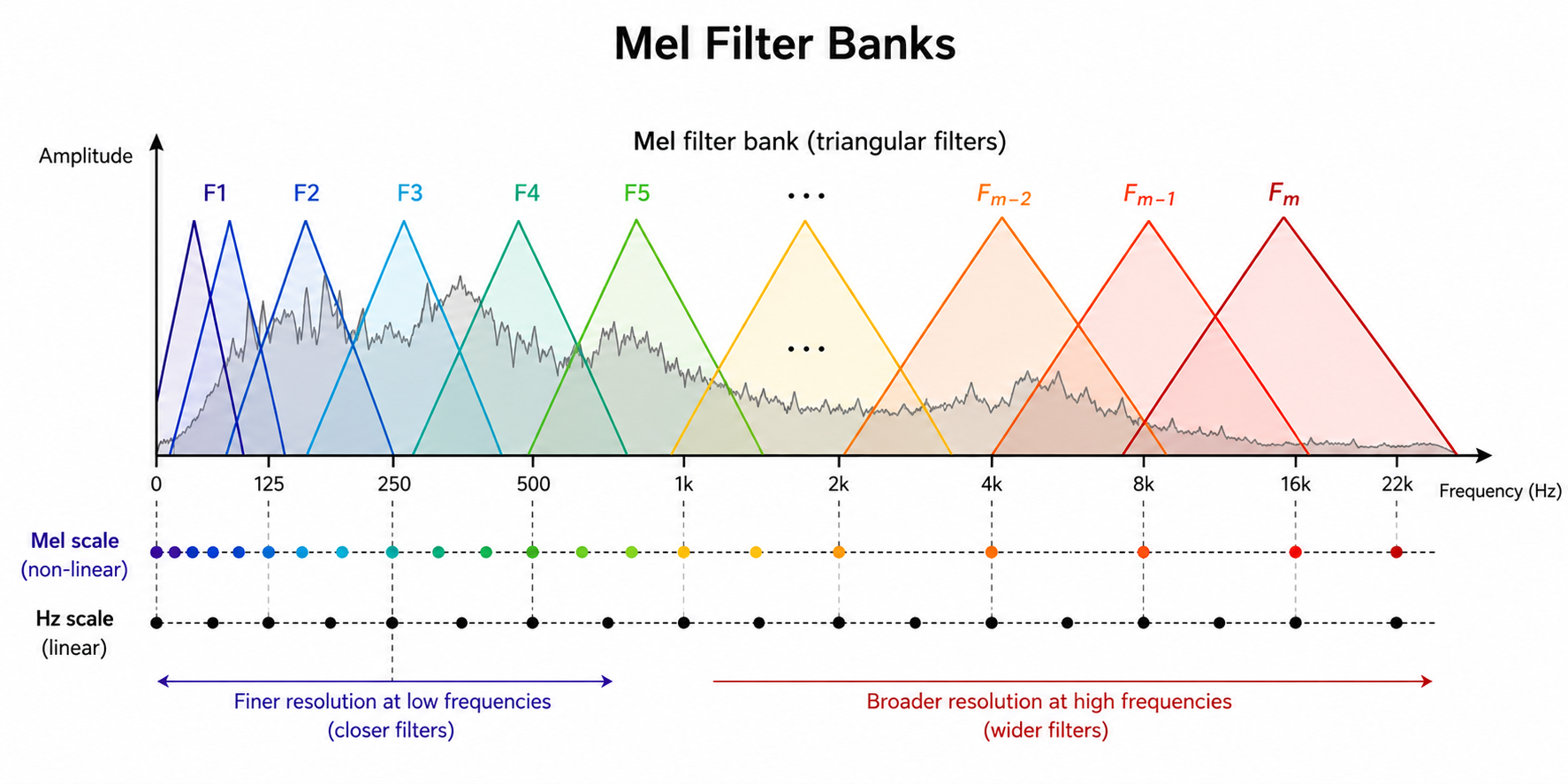
Suppose we have $M$ Mel filters. For each short-time frame of the audio signal, the energy in each filter can be calculated. If the magnitude or power spectrum is represented by $S[k]$, then the energy associated with the $m$-th filter can be written conceptually as

where $H_m[k]$ represents the $m$-th Mel filter.

The result is a much smaller representation of the original spectrum. Instead of retaining every frequency bin, we summarize the spectral energy into perceptually motivated frequency regions.

This is an important recurring theme in signal processing: we trade some information for a representation that may be more useful for the problem at hand.

Why Use Mel Spectrograms?

You might reasonably ask: why throw away information? If the Fourier Transform gives us all those beautiful frequency bins, why not simply keep everything?

The answer is that more information is not always the same thing as more useful information.

A raw spectrogram contains detailed frequency information, much of which may not be equally important for human perception or for a particular machine learning task. The Mel representation compresses the frequency axis while preserving a broad structure that is relevant to how humans hear.

There is also a computational advantage. A typical spectrogram can contain hundreds or thousands of frequency bins. A Mel spectrogram may summarize this information using a much smaller number of Mel bands, such as 40, 64 or 128.

So we have moved from

Waveform $\rightarrow$ STFT $\rightarrow$ Spectrogram $\rightarrow$ Mel filter bank $\rightarrow$ Mel spectrogram

Each step introduces another layer of abstraction.

But What About Loudness?

There is another perceptual property we should consider. Remember amplitude from Part 1? We said that amplitude is an objective property of the signal, while loudness is a perceptual experience. The same idea appears again here.

The amplitude or power of a frequency component can vary over several orders of magnitude. If we simply display these values linearly, weaker components may be almost invisible compared with stronger ones.

This is why audio processing often uses a logarithmic scale for spectral energy. A common representation is the decibel scale:

where $P$ is the measured power and $P_0$ is a reference power.

If we are working with amplitude rather than power, the corresponding expression is commonly written as

The logarithm is useful because human perception of intensity is also approximately logarithmic over substantial ranges. Again, this is not a statement that the human auditory system literally computes a logarithm. Rather, logarithmic representations are useful approximations for handling the enormous dynamic ranges encountered in audio.

From Mel Spectrograms to MFCCs

We now have a representation that captures the evolution of perceptually motivated spectral energy over time. But audio researchers were not finished yet. We can go one step further.

One of the most influential feature representations in speech processing is the Mel-Frequency Cepstral Coefficient, commonly abbreviated as MFCC.

The name sounds considerably more intimidating than the underlying idea.

The basic MFCC pipeline can be summarized as:

Waveform $\rightarrow$ Pre-emphasis $\rightarrow$ Framing $\rightarrow$ Windowing $\rightarrow$ FFT $\rightarrow$ Power Spectrum $\rightarrow$ Mel Filter Bank $\rightarrow$ Log Energy $\rightarrow$ DCT $\rightarrow$ MFCCs

Some modern implementations may omit or modify parts of this traditional pipeline, but this sequence captures the classical formulation.

We have already discussed most of these components. Framing and windowing are related to the STFT. The FFT gives us the frequency representation. The Mel filter bank gives us perceptually motivated frequency bands, and the logarithm compresses the dynamic range.

So what is left?

The Cepstrum: A Spectrum of a Spectrum?

This is where the terminology becomes wonderfully strange.

After obtaining the log Mel energies, we apply the Discrete Cosine Transform (DCT). The resulting coefficients are the MFCCs.

The DCT can be thought of, at a high level, as another transformation that represents the pattern of the log spectral energies using a smaller number of coefficients. The lower-order coefficients capture broad spectral shape, while higher-order coefficients capture progressively finer variations.

The term "cepstrum" itself is a playful inversion of the word "spectrum." It emerged from the idea of analysing the structure of a spectrum in another transformed domain. Do not worry if this sounds slightly circular. Signal processing people have a strange sense of humour.

The important practical idea is that MFCCs provide a compact representation of the spectral envelope of a sound, and this representation became extremely useful in speech recognition and other audio classification tasks.

Why Are MFCCs Useful for Speech?

Human speech contains a tremendous amount of information. The vocal folds provide an excitation source, while the vocal tract shapes that excitation through resonances. These resonances create concentrations of acoustic energy at particular frequencies known as formants.

The exact pattern of these resonances changes as we move between different vowels and speech sounds. Consequently, the spectral envelope contains valuable information about the configuration of the vocal tract.

MFCCs provide a compact way of representing this spectral envelope. Historically, this made them extremely useful for speech recognition systems, speaker recognition, emotion recognition and many other audio-processing problems.

This is another beautiful example of domain knowledge being transformed into a computational representation. Instead of giving a machine learning algorithm the entire raw acoustic signal and asking it to discover everything from scratch, we can construct a representation that incorporates assumptions about the physics of speech production and the perception of sound.

Are MFCCs Still Relevant in the Deep Learning Era?

Now comes the obvious question. If MFCCs are so useful, why do modern deep learning systems increasingly operate directly on waveforms or spectrograms? Are MFCCs obsolete?

Not really.

MFCCs remain useful in many applications, especially where computational efficiency, interpretability or relatively small datasets matter. They are also an excellent example of how decades of signal-processing research distilled knowledge about speech into a compact feature representation.

However, modern deep learning has changed the game. Large neural networks can learn increasingly sophisticated representations directly from waveforms or time-frequency representations. Models can discover patterns that traditional hand-designed features may discard.

This creates an interesting tension between representation engineering and representation learning.

Traditional signal processing asks:

"What representation should we construct using what we already know about the signal?"

Deep learning often asks:

"What representation can the model learn from the data itself?"

In reality, modern systems often combine both ideas. Even when a model learns from relatively raw inputs, architectural choices, preprocessing, normalization, sampling rate, windowing and other design decisions still encode assumptions about the underlying signal.

Putting It All Together

Let's step back for a moment.

In Part 1, we started with physics. A vibrating object produces pressure variations that propagate through a medium. In Part 2, we converted those physical phenomena into numbers using microphones, sampling and quantization. In Part 3, we learned how to look at those numbers from another perspective using Fourier analysis and the spectrogram.

Now, in Part 4, we introduced the human being back into the equation.

The physical frequency of a signal is measured in Hertz, but human perception of frequency is not perfectly linear. The Mel scale provides one perceptually motivated way of representing frequency. Applying Mel-spaced filter banks to a spectrogram produces a Mel spectrogram, which gives us a compact representation of spectral energy that roughly reflects aspects of human auditory perception.

Taking this one step further, logarithmic compression and the Discrete Cosine Transform lead us to MFCCs, one of the classical feature representations that shaped decades of speech and audio processing research.

Physical Sound $\rightarrow$ Analog Signal $\rightarrow$ Digital Waveform $\rightarrow$ Fourier Transform $\rightarrow$ Spectrogram $\rightarrow$ Mel Spectrogram $\rightarrow$ MFCC

Look at how many layers of abstraction we have accumulated. Yet at the bottom of this entire stack is still the same thing: a vibrating physical system creating pressure variations in a medium.

This is precisely why I find signal processing so fascinating. We can progressively transform a phenomenon from one representation into another, each representation revealing something different about the underlying system. There is no single representation that is universally "correct." The usefulness of a representation depends on the question we are trying to answer.

And this brings us very close to machine learning.

We now have a waveform. We have a frequency representation. We have a spectrogram. We have a Mel spectrogram. We have MFCCs. We can therefore begin asking a very different question: can a machine learn to recognize patterns in these representations?

That is where the story becomes particularly interesting.

In the next part, we will finally begin connecting these representations to machine learning. We will explore how audio can be framed as a supervised learning problem, how features become inputs to models, why spectrograms can be treated almost like images, and how convolutional neural networks entered the world of audio.

The rabbit hole continues.

See you in Part 5.