Author: Yusuf Brima

Introduction

In today’s data-driven world, uncovering hidden structures within complex datasets is a crucial task, whether it’s analyzing customer behavior, identifying disease patterns in medical data, or classifying text documents. Machine learning (ML) algorithms offer powerful tools to navigate the intricacies of data analysis. Boardly speaking, these ML algorithms can be categorized into Supervised Learning, Unsupervised Learning, and Reinforcement Learning. In this post, we will focus on the unsupervised learning algorithm, K-means clustering. This algorithm has recently gained traction in the field of representation learning also know as feature learning, where it is used to learn a representation of the data. This versatile technique has found applications in various domains, addressing challenges like market segmentation, anomaly detection, image recognition, and recommendation systems. By automatically identifying groups of similar data points based on their features, K-means clustering enables efficient customer segmentation, personalized healthcare approaches, and effective text categorization. It leverages computational power to unveil valuable patterns and provides insights that may not be apparent at first glance, empowering businesses, researchers, and analysts to make informed decisions and drive innovation.

Therefore, in this post, we will discuss the underlying principles of the K-means clustering algorithm including it’s mathematical derivation and a step-by-step implementation in Python. We will also discuss the limitations of the algorithm and provide pointer to resources for further reading.

Measuring Distance

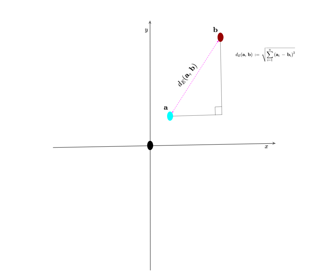
However, to start, we must first build an inuition of measuring distances between points because this is very important in the K-means clustering and other machine learning algorithms. In this post, we will focus on the Euclidean distance, which is the most common distance metric used in machine learning. The Euclidean distance between two points, $x$ and $y$, in an $n$-dimensional real vector space is defined as the square root of the sum of the squared differences between the corresponding elements of the two vectors. The Euclidean distance can be expressed as follows:

where $x_i$ and $y_i$ are the $i$th elements of the vectors $x$ and $y$, respectively. The Euclidean distance is also known as the $L_2$ norm or $L_2$ distance. I have illustrated this concept in Figure 1 below.

Now that we have a basic intuition of measuring distances between points, we can now discuss the K-means clustering algorithm.

The underlying principles

The goal of $K$-means clustering is to group similar data points together based on their features. In this algorithm, we start with an initial guess of $K$ centroids (centers of mass) of the clusters and then iteratively assign each data point to the nearest centroid based on a distance metric such as Euclidean distance in equation $\ref{eq:Euclidean_Distance}$ and update the centroid based on the mean of the assigned data points.

The $K$-means algorithm is initialized with the number of clusters, $K$, and the initial centroids are chosen randomly or using some other heuristic approach. Once the initial centroids are chosen, the algorithm alternates between two steps until convergence:

1. Assignment step: In this step, each data point is assigned to the nearest centroid. Specifically, each data point is assigned to the cluster with the nearest centroid based on the Euclidean distance or other distance metric. The assignment step can be formulated as follows: \(\begin{equation} c_i = d_D(\mathbf{x}_i, \boldsymbol{\mu}_j) \end{equation}\) where $\mathbf{x}_i$ is the $i$-th data point, $\boldsymbol{\mu}_j$ is the centroid of the $j$-th cluster, and $c_i$ is the index of the cluster that the $i$th data point is assigned to.
2. Update step: In this step, the centroids are updated based on the mean of the data points assigned to each cluster. The update step can be formulated as follows:

where $n_j$ is the number of data points assigned to the $j$th cluster, $\delta_{c_i,j}$ is the Kronecker delta which is 1 if $c_i=j$ and 0 otherwise, and the sum is taken over all $n$ data points.

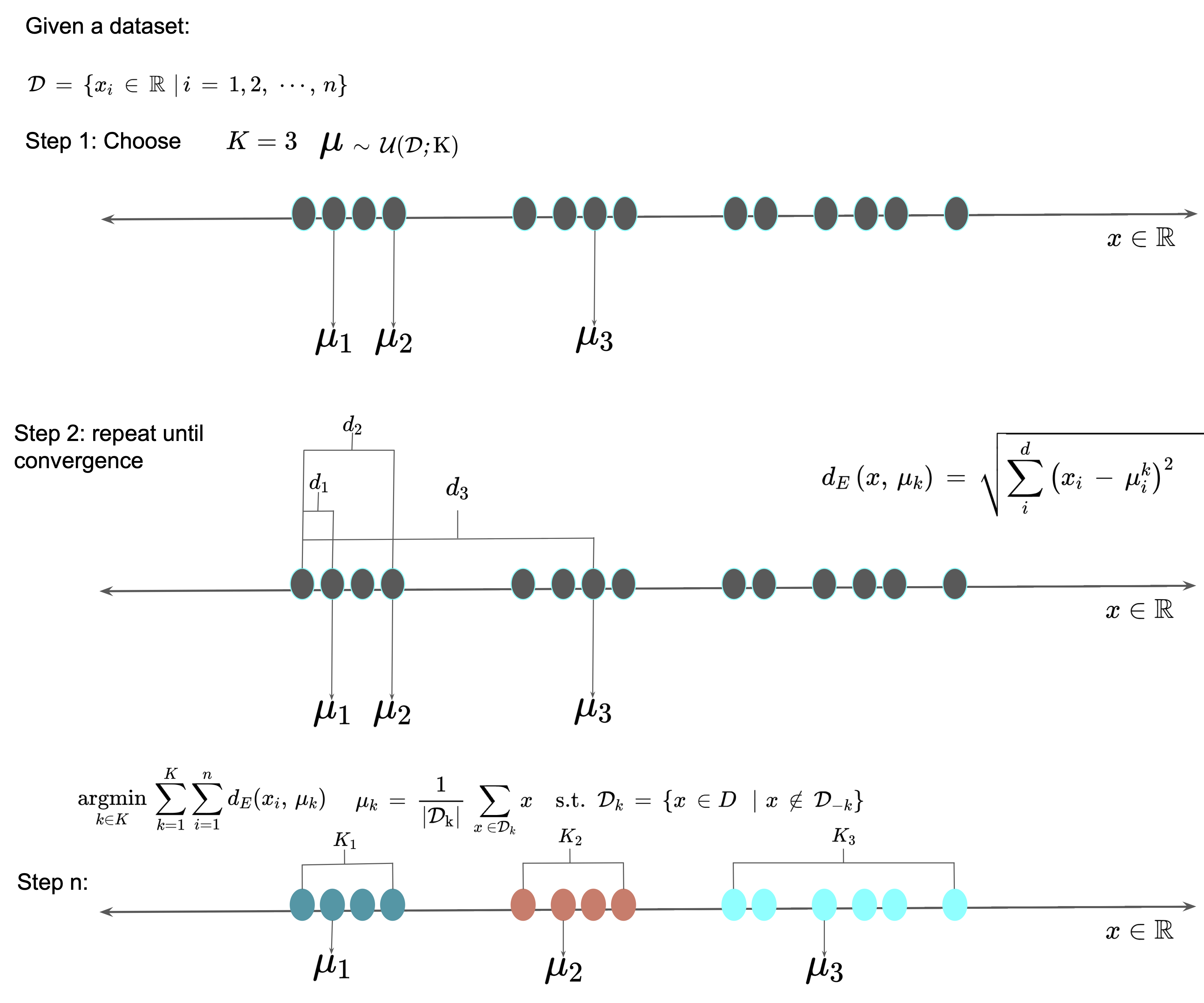
The algorithm iterates between these two steps until convergence, which is typically determined by a stopping criterion such as a maximum number of iterations or when the change in the centroids falls below a certain threshold. We have shown an illustration of this approach to clustering of a $2D$ feature space in Figure 2.

Implementation in Python

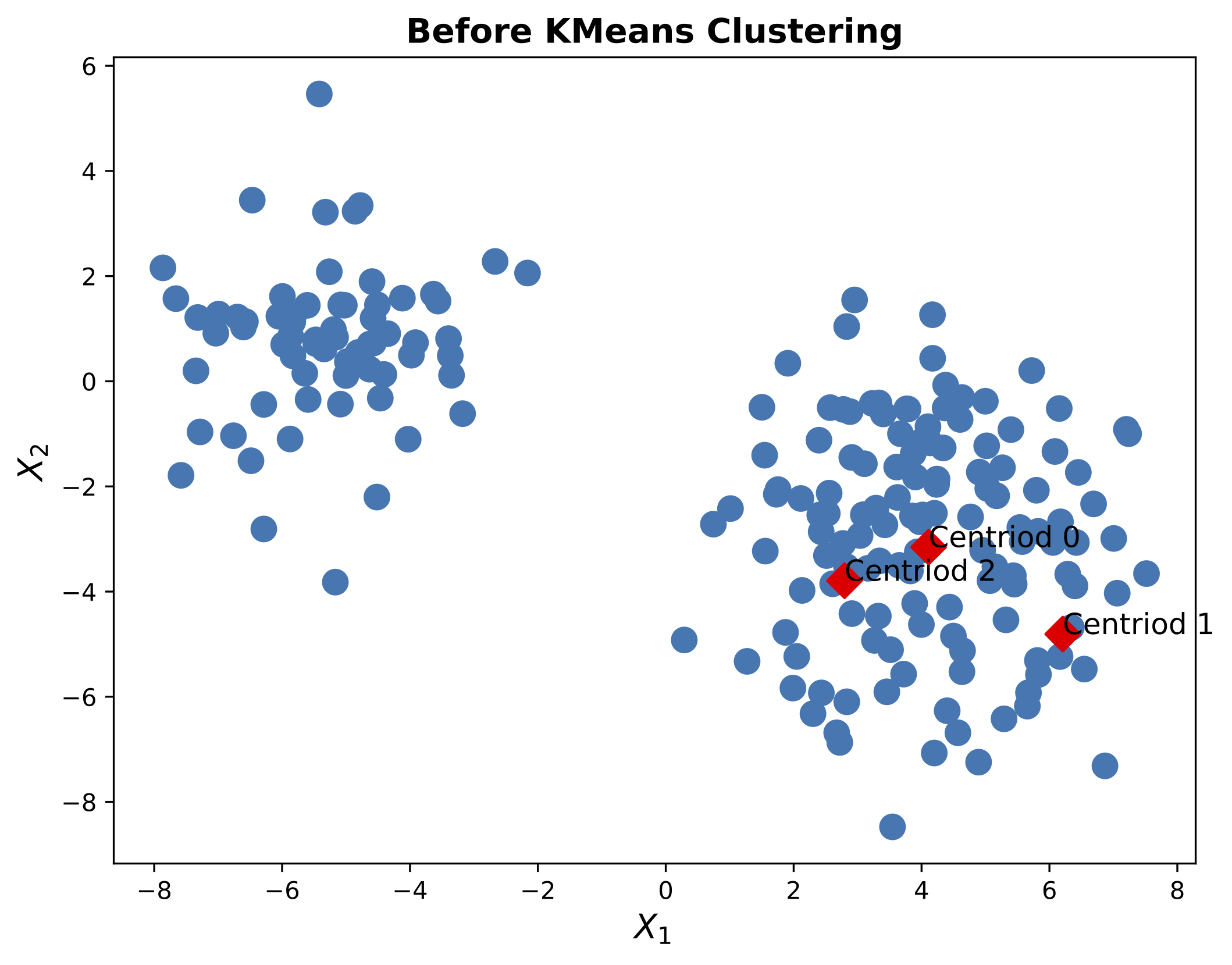
We will now implement the $K$-means clustering algorithm in Python. We will use the make_blobs function from the sklearn.datasets module to generate a synthetic dataset with 200 samples and 2 features. The make_blobs function generates isotropic Gaussian blobs for clustering. We will set the random_state parameter to 123 to ensure reproducibility of the results. We will also plot the data to visualize the clusters.

We first import the necssary modules and set the seed for reproducibility.

import numpy as np
import matplotlib.pyplot as plt
import sklearn.datasets as ds
import random 
# set the seed
random.seed(123)
np.random.seed(123)

Then we generate the datapoints

# make blobs
X, y = ds.make_blobs(n_samples=200, centers=3, n_features=2, random_state=123, cluster_std=1.5, random_state=123)
K = 3

We choose the inital centriod.

# We choose K random points as initial centroids
idx =  np.random.choice(X.shape[0], K, replace=False)
centroids = X[idx, :]

We can now plot the data to visualize the clusters.

# plot the blobs
plt.figure(figsize=(8,6))
scatter  = plt.scatter(X[:,0], X[:,1],s=100)
plt.scatter(centroids[:,0], centroids[:,1], c = 'red', marker = 'D', s = 100)
# add text to the centroids
for i in range(K):
    plt.text(centroids[i,0], centroids[i,1], f"Centriod {str(i)}", fontsize=12)

plt.xlabel(r"$X_1$", fontsize=14)
plt.ylabel(r"$X_2$", fontsize=14)
plt.title("Before KMeans Clustering", fontsize=14, fontweight='bold' )
plt.savefig("KMeans_Before_Clustering.pdf", dpi=300, bbox_inches='tight', pad_inches=0.1)
plt.show()

Here, were have chose $K=3$, meaning we have three clusters. We can visualize the data using a scatter plot as shown in Figure 3.

The next step is to define three helper functions (euclidean_distance, evaluate_point, KMeans). The euclidean_distance function computes the Euclidean distance between two points. The evaluate_point function assigns a point to the closest centroid. The KMeans function implements the $K$-means clustering algorithm. The KMeans function takes the data, the number of clusters, and the maximum number of iterations as input. The function returns the cluster assignments and the cluster centroids.

def euclidean_distance(x1, x2):
    return np.sqrt(np.sum((x1 - x2)**2))


def evaluate_point(point, centroids):
    distances = [euclidean_distance(point, centroid) for centroid in centroids] # This operation performs a list comprehension to compute the distance between the point and each centroid
    closest_centroid = np.argmin(distances) # This operation returns the index of the closest centroid
    return closest_centroid

# Manual KMeans
def KMeans(X, K, max_iter = 100):
    c_idx =  np.random.choice(X.shape[0], K, replace=False) # randomly choose the initial centroids
    centroids = X[c_idx, :] # assign the initial centroids
    for i in range(max_iter): # iterate over the maximum number of iterations
        # assign the points to the closest centroid
        clusters = [evaluate_point(point, centroids) for point in X] # This operation performs a list comprehension to assign each point to the closest centroid
        clusters = np.array(clusters) # convert the list to a numpy array
        # update the centroids
        for i in range(K):
            idx = np.where(clusters == i)
            centroids[i] = X[idx , :].mean( axis = 1)
    return clusters, centroids

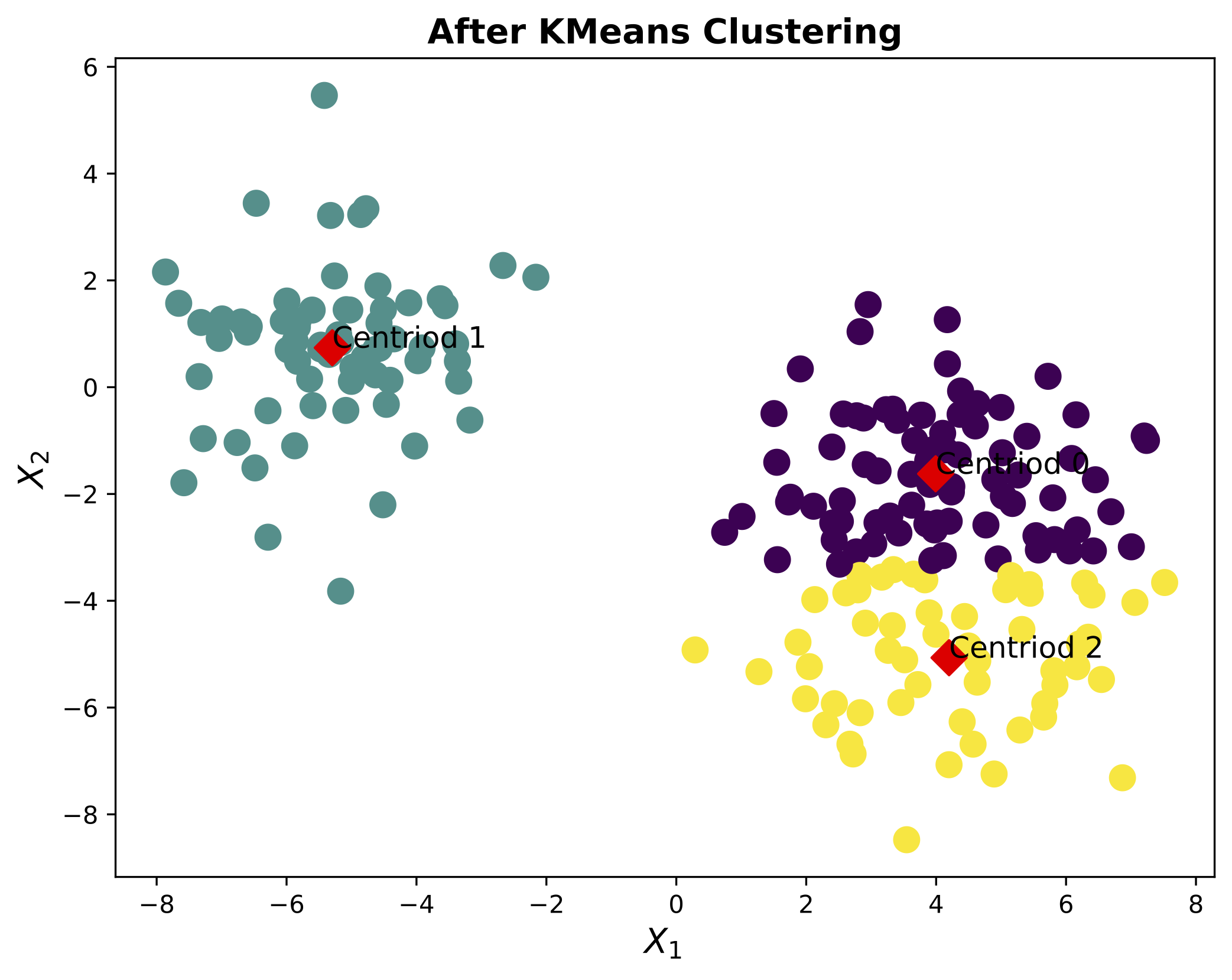
With these helper functions, we can now implement the $K$-means clustering algorithm. We will use the KMeans function to cluster the data. We will set the maximum number of iterations to 100. We will also plot the data to visualize the clusters.

clusters, centroids = KMeans(X, K, max_iter = 100)

We can now plot the data to visualize the clusters.

# plot the blobs
plt.figure(figsize=(8,6))
scatter  = plt.scatter(X[:,0], X[:,1],s=100, c = list(clusters)) 
plt.scatter(centroids[:,0], centroids[:,1], c = 'red', marker = 'D', s = 100)
# add text to the centroids
for i in range(K):
    plt.text(centroids[i,0], centroids[i,1], f"Centriod {str(i)}", fontsize=12)


plt.xlabel(r"$X_1$", fontsize=14)
plt.ylabel(r"$X_2$", fontsize=14)
plt.title("After KMeans Clustering", fontsize=14, fontweight='bold' )
plt.savefig("KMeans_After_Clustering.pdf", dpi=300, bbox_inches='tight', pad_inches=0.1)
plt.show()

The data is plotted in Figure 4.

Putting this all together, we have the following code.

In conclusion, we have implemented the $K$-means clustering algorithm from scratch. We have also used the algorithm to cluster a synthetic dataset. This is purely for a learning purpose to deepen ones understanding of how and why the algorithm works. In practice, libraries such as scikit-learn should be used to implement the $K$-means clustering algorithm.

K-means clustering is a computationally efficient algorithm and can handle large datasets. However, its performance can be sensitive to the initial choice of centroids and the number of clusters. Additionally, k-means clustering assumes that clusters are spherical and equally sized, which may not always be the case in practice.

Our future will continue with other representation learning algorithms such as K-Nearest Neighbours, PCA, ICA, Auto Encoders etc. So, stay tuned. Happy learning!

Acknowledgement

Thanks to Dr. Ulf Krumnack for his insightful feedback while developing this post.