Author: Yusuf Brima

Introduction

In this post, I will walk through how to implement the K-Nearest Neighbors (K-NN) machine learning algorithm from scratch in Python. K-NN is one of the most fundamental ML algorithms used for classification and regression.

Understanding KNN

The intuition behind K-NN is quite simple. Given a new data point, let us call it $X_\textrm{new}$, one look at its closest $K$ neighbors in the training data and predict the label based on those neighbors. For classification, take a majority vote of the neighbor labels. For regression, take the average of the neighbor values.

Here are the steps to follow to apply K-NN:

1. Choose a value for $K$ - the number of neighbors to examine.
2. Calculate the distance between the new data point and all points in the training set using a distance metric like Euclidean or Manhattan distance.
3. Sort the distances and take the top $K$ closest points.
4. For classification, take the majority class label of the $K$ points. For regression, take the average value of the K points.

An illustration of the K-NN algorithm for a sample 2D dataset is shown below:

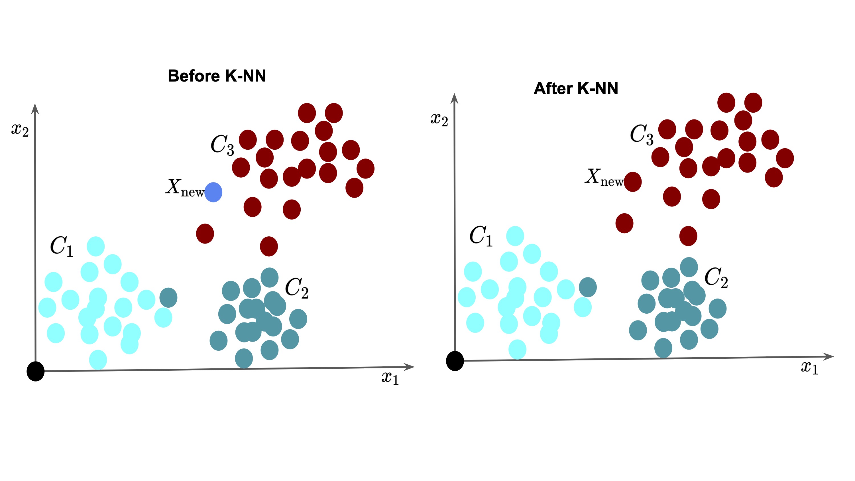
The key steps are computing distances, finding neighbors, and aggregating labels. The effectiveness of K-NN depends heavily on the choice of distance metric and value of $K$.

Implementing K-NN Classifier in Python

I will now walk with you through a simple example of implementing a K-NN classifier in Python for classifying 2D points.

First, we generate some sample 2D data:

import numpy as np
from sklearn.datasets import make_blobs

X, y = make_blobs(n_samples=500, centers=2, random_state=42)

For 2D data, I use the Euclidean distance metric.

The Euclidean distance between two points a and b is:

Where:

• $a = (a_1, a_2, …, a_n)$
• $b = (b_1, b_2, …, b_n)$
• $a_i, b_i$ are the $i$-th components of vectors a and b
• $n$ is the dimensionality of the space Using summation notation makes the equation more compact and generalizable to any number of dimensions.

The implementation is straightforward using a loop. We can use advanced linear algebra techniques which are more efficient for high-dimensional data to achieve the same but I’ll skip that for the sake of simplicity since we are in 2D and number of samples is relatively small:

import math

def euclidean_distance(a, b):
  distance = 0
  for i in range(len(a)):
    distance += (a[i] - b[i])**2
  return math.sqrt(distance) 

To find the $K$ nearest neighbors, we calculate distances to all points, sort them, and take the first $K$:

import operator

def get_neighbors(training_set, new_point, K):
  distances = []
  for x in training_set:
    dist = euclidean_distance(x, new_point)
    distances.append((x, dist))

  distances.sort(key=operator.itemgetter(1))
  
  neighbors = []
  for x in range(K):
    neighbors.append(distances[x][0])
    
  return neighbors

For classification, we take a majority vote among the $K$ neighbors:

import collections

def predict_classification(training_set, new_point, K):
  neighbors = get_neighbors(training_set, new_point, K)
  output_values = [x[-1] for x in neighbors]
  prediction = collections.Counter(output_values).most_common(1)[0][0]  
    
  return prediction

And we have a basic K-NN classifier in Python! With just a few lines of code and have implemented the core ideas behind K-NN - computing distances, finding neighbors, and aggregating their labels. Next you may wonder, how do we get to choose $K$ and the distance metrics? Stay with me, we are delving into this right away.

Choosing $K$ and Distance Metrics

The two most important design choices with K-NN are selecting the value of $K$ and the distance metric. Finding the optimal values requires experimenting on a validation set.

Here are some guidelines on choosing $K$ and distance metrics:

• $K$ controls the tradeoff between bias and variance. Larger $K$ reduces variance but increases bias. Hyperparameter optimization can help choose the ideal $K$.
• Distance metrics depend on the data type. Euclidean works best for low dimensions. Manhattan or Hamming are better for high dimensions.
• Feature scaling is important before computing distances.
• For weighted features, use a weighted distance like Mahalanobis distance.

When does K-NN Shines?

K-NN tends to perform very well when:

• The data has low inherent dimensionality, meaning number of idenpendent variables is relatively small like our examples shown here.
• The decision boundaries between classes are irregular.
• There is plentiful training data compared to dimensionality, meaning number os training samples is much much greater than the independent variables, tabular data for examples on customer data.

When does K-NN struggle?

• Data has very high dimensionality curse of dimensionality
• Classes are well-separated
• Training data is sparse
• Need to extrapolate beyond training data

In many cases, other algorithms like SVM, random forests, and neural nets outperform K-NN, especially on complex modern datasets. But K-NN is still widely used for its simplicity, interpretability, and surprisingly good performance.

Summary

In this post, I walked through implementing K-Nearest Neighbors from scratch in Python based on first principles. K-NN exemplifies the powerful “learning by analogy” paradigm underlying many ML algorithms. With just distances and neighbors, K-NN can deliver excellent results on many problems while being simple to understand and implement. While more complex techniques like deep nets are popular today, starting with fundamentals like K-NN is key for any practitioner looking to really grok machine learning.