
Understanding Sound from First Principles
Published:
Author: Yusuf Brima
Introduction
Welcome. We are going to embark on a journey, together, of course in gaining a deeper intuition of sound and it's general applications to machine learning problems from simple toy use cases like instrument classification to advance Music Information Retrieval (MIR). This is going to be a series of post that will delve into the mysterious world of sound and it's ubiquity of application This blog is greatly inspired by Valerio Velardo, who continues to lower the learning curve of Machine Learning in the audio space. Yes, you are right to be wondering how for heaven's sake (assuming you believe in one), I ended up here talking my head about audio. Well, it's a long story and it's best we save the details for another day! I was recruited into a PhD programme in Computational Cognition at Universität Osnabrück Institute of Cognitive Science where state-of-the-art ML tools need to be used in automating information processing: from vocal signature analysis to speaker diarization and everything in between. So, that was my journey to the great awakening in this world of Audio Signal Processing and Machine Learning, yes not just Deep Learning. Justifications will clear later on.
What is sound?
Have you heard of the famous quote by Nikola Tesla: “If you wish to understand the Universe think of energy, frequency and vibration.“ I have a tingling he was right. If we take a multi-scale view of everything around us, from the macrocosmic view of the spiral expanding universe to the wiggling dance of subatomic participles at the Planck scale, these three phenomena are at play all the time. And so you may be wondering how does that relate to sound. Well, it certainly does relate to sound in every way one could imagine. A sound is created when a physical system vibrates. This vibration may be caused when a physical system is displaced from its equilibrium condition and is allowed to respond to the forces that tend to restore its equilibrium. A simple manifestation of Isaac Newton's laws of Motion. This vibration causes a differential change in air pressure around the local region that produced the vibration. The pressure oscillates and propagates in the medium where the vibration occurred for example through the air. Thus, sound is a wave, a longitudinal wave that carries energy. But a wave is a disturbance of a medium (e.g., air) which transports vibrational energy through the medium without permanently transporting matter. This is very important because in a wave, temporarily displaced particles of the medium return to rest when the energy dissipates through a fancy notion in physics know as a restoring force. And example of this concept is shown in Figure 1 below.
When a physical system is at rest (i.e., all net forces such as gravity, push or pull of a spring, acting on the body are balanced meaning they sum up to 0). Then the body is in an equilibrium state. However, a nudge on an object at equilibrium will tend to cause to system to vibrate proportionally to the applied force. This is the basis of oscillation, resonance, and waves, which are the crux of of studying sound consequently AI audio as shown in Figure 2. But, let's don't get ahead of ourselves because the jigsaw puzzle is not solved yet completely. To truly understand the theoretical basis of sound we need to traverse the landscapes of signal processing and a bit of information theory. These two fields lay the basis of studying the underlying foundations of signal processing (analog and digital) and information flow in the modern era of computing.
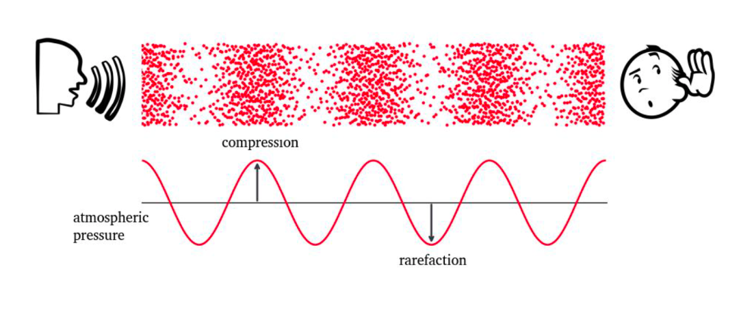
So far we have stated that sound is a result of a vibrating system causing a ripple of longitudinal waves that causes compression and rarefaction of air molecules in local regions thus propagating sound energy. Next, we are going to explore a simple notion of this concept using a Sine Wave as shown in equation \ref{eq:wave_form}. But before that we need to solidify our knowledge of frequency, amplitude, period and phase of a signal in general (continuous or discrete in time or frequency) but more specifically to sound because that is where our interest lies.
The frequency $f$ as shown in equation \ref{eq:frequency}, is the number of cycles in a unit time (often shown in cycles per second). It is measures how often something happens (causally speaking). We measure frequency in Hertz named after the German physicist Heinrich Rudolf Hertz. As we will see later, the frequency has a great role to play in audio signal processing. As nice characteristics of the frequency is shown in the animation on Figure 3 (Left). Where the sine wave is shown for varying frequencies. Some of these really look cool: the symmetry the create is mesmerising!
$$ \begin{equation} f = \frac{1}{T} \label{eq:frequency}, \end{equation} $$The period $ T $ as shown in equation \ref{eq:period}, measures the time it takes for a given frequency to complete a cycle. As as time quantity, it is measured is seconds (s). And it is inversely proportional to $f$. This means, if we increase the frequency, it consequently leads to a shorter period and vice versa. You get the idea. $$ \begin{equation} T = \frac{1}{f} \label{eq:period}. \end{equation} $$
Next we will talk about the amplitude of a wave. Remember our animation from Figure 1. Great. The amplitude measures the magnitude of a signal. It gives us information how far, by any notion of the the word far, we are from the time axis along the y-axis. If you're think about loudness, that is very close, because amplitude and loudness have a unique relation. However, loudness is subjective and depends on many factors such as age, distance, medium e.t.c., will amplitude is objective. Finally, we have the phase $\varphi \in [0,1]$ as in the equation below. Which measures the deviation of the signal from the origin. This shown as a flowing river in Figure 3 (Right) where different phase values displace the signal from the origin. Thus when a continuous wave is sampled and quantized we are actually measuring all these traits and more as a function of time.
$$ \begin{equation} y(t) = A \sin \left( 2 \pi f t + \varphi \right) \label{eq:wave_form} \end{equation} $$ Where $A$ is the amplitude, $f$ is the frequency, $t$ is the period and $\varphi$ is the phase of the signal.
That's all for now. In the next post, we will talk about periodic and aperiodic signals as well as sound acquisition in digital systems. See Part 2 where we talk about sound acquition from analog to digital systems
Leave a Comment