Approximation Theory (for newbies)

If you're new to this series, please checkout our previous post on the fundamentals then head back here after getting your feet wet.

In Part I, we spent a good deal of time falling in love with the elegance of closed-form (analytical) solutions to differential equations. We separated variables, hunted for integrating factors, and even flirted with exactness. That's all well and good, and if you followed along, odds are you can now solve a fair number of first and second order ODEs by hand. However (and this is the part nobody warns you about at the start), most differential equations that show up in the wild flatly refuse to be tamed this way. The Lotka-Volterra equations we teased in Part I do not, in general, admit a closed-form solution written in terms of elementary functions. Neither does the Lorenz system, nor most realistic versions of the SIR model once you complicate them even slightly. So, what do we do when pen, paper and cleverness are not quite enough? We approximate!

This is where numerical methods enter the story. Instead of insisting on an exact formula $y(x)$ that satisfies our differential equation everywhere, we settle for a good estimate of $y$ at a discrete set of points $x_0, x_1, x_2, \ldots, x_n$. If we choose our step size wisely, and if our method is sound, this sequence of estimates traces out a curve that hugs the true solution closely enough to be genuinely useful. It won't be exact, but as engineers, scientists and generally practical people, we can live with that.

Euler’s Method: Our First Numerical Solver

The simplest, and historically the first, numerical method for solving ODEs is Euler's method, named after the very same Leonhard Euler whose notation we admired in Part I. The idea is disarmingly simple, so simple in fact that you may wonder why we bothered with all that separation of variables business at all. Bear with us though, because simplicity comes at a price, as we shall soon see.

Geometric Intuition

Recall the generic first order ODE from Part I:

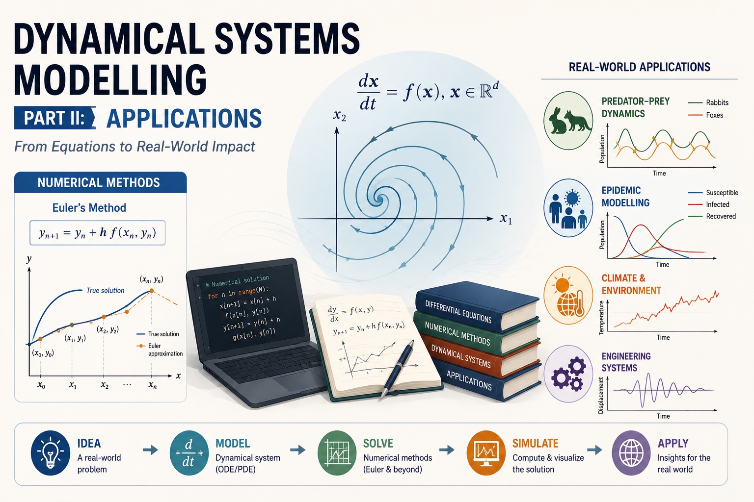
with initial condition $y(x_0) = y_0$. Geometrically, $f(x_0, y_0)$ is nothing more than the slope of the solution curve at the point $(x_0, y_0)$. If we don't know where the curve goes next, the next best thing is to assume it keeps going in a straight line along that slope, at least for a little while. So we take a small step of size $h$ along that tangent line, land at a new point, recompute the slope there, and repeat. It's a bit like feeling your way down a dark hallway one small step at a time, using only the direction you're currently facing.

The Algorithm

Formally, if we let $x_{n+1} = x_n + h$, Euler's method gives us the following update rule:

Starting from $(x_0, y_0)$, we apply equation $\ref{eq:euler}$ repeatedly, generating a sequence of approximations $y_1, y_2, y_3, \ldots, y_n$ at the points $x_1, x_2, x_3, \ldots, x_n$. Notice that equation $\ref{eq:euler}$ generalizes rather nicely to the vector form of the ODE we introduced right at the start of Part I, equation $\dot{\mathbf{x}} = f(\mathbf{x})$, simply by letting $\mathbf{y}_{n+1} = \mathbf{y}_n + h\, f(\mathbf{y}_n)$. This little observation is not a footnote; it's the reason Euler's method (and its descendants) can just as easily march forward a single population count or an entire system of coupled equations. We'll lean on this fact later.

Example: Revisiting the Rabbits

Let's return to our rabbit population from Part I, governed by $\frac{dN}{dt} = rN$, with $r = 0.01$ new rabbits per week per current rabbit, and $N(0) = 1000$. Using a step size of $h = 1$ week, equation $\ref{eq:euler}$ becomes $N_{n+1} = N_n + h \, r \, N_n$. Let's crank the handle a few times:

• $N_1 = 1000 + (1)(0.01)(1000) = 1010$
• $N_2 = 1010 + (1)(0.01)(1010) = 1020.1$
• $N_3 = 1020.1 + (1)(0.01)(1020.1) = 1030.301$

Now, you may recall from Part I that this equation actually has a lovely closed-form solution, $N(t) = N_0 e^{rt}$. At $t = 3$, this gives us $N(3) = 1000 \, e^{0.03} \approx 1030.455$. Our Euler estimate of $1030.301$ is close, but not exact, off by about $0.15$ rabbits. Not a catastrophe for rabbits, but you can imagine how such small errors, accumulated step after step over a long simulation, might eventually matter a great deal.

How Good (or Bad) is Euler's Method?

The gap we just observed is no accident, it's baked into the method itself. Because Euler's method approximates a curved solution using straight tangent-line segments, it commits an error at every single step, called the local truncation error, which can be shown (via a Taylor expansion of $y$ around $x_n$) to be of order $O(h^2)$. Accumulated over the roughly $\frac{1}{h}$ steps needed to cover a fixed interval, the total, or global error, works out to $O(h)$. In plain English, halving the step size roughly halves the overall error. This makes Euler's method what mathematicians call a first order method. It is wonderfully easy to understand and to code, but it is, frankly, a bit of a blunt instrument. Thankfully, we can do better without much extra effort.

Improving on Euler: Heun’s Method

The trouble with Euler's method is that it commits to the slope at the beginning of the step and never looks back, even though the slope is clearly changing as we move across the interval. A natural fix, and one of the oldest tricks in the numerical analysis book, is to compute the slope at both ends of the step and average the two. This is precisely the idea behind Heun's method, sometimes called the improved Euler method, or a predictor-corrector method.

First, we take a normal Euler step to predict where we might end up:

Then, we use this predicted point to correct our estimate, by averaging the slope at the start of the step with the slope at our predicted endpoint:

Let's put this to work on our rabbits, one more time. With $N_0 = 1000$, the predictor gives us $N_1^{*} = 1000 + (1)(0.01)(1000) = 1010$, exactly as before. Now the corrector kicks in:

Compare this to the exact value $N(1) = 1000\,e^{0.01} \approx 1010.0502$. That's remarkably close, and it didn't cost us much more computation than Euler's method. This improvement in accuracy is not a coincidence either; it can be shown that Heun's method has a local truncation error of $O(h^3)$ and a global error of $O(h^2)$, earning it the title of a second order method. Halving $h$ now quarters the error, which is a much better trade for our computational effort.

The Workhorse: Fourth Order Runge-Kutta

If Euler's method is a bicycle and Heun's method is a scooter, then the fourth order Runge-Kutta method, affectionately known as RK4, is the reliable family car of numerical ODE solving. It remains, to this day, one of the most widely used general-purpose methods, striking a comfortable balance between accuracy and computational cost. The idea again is to sample the slope $f$ at several cleverly chosen points within the step and combine them in a weighted average.

Specifically, for the ODE in equation $\ref{eq:generic_ode}$, RK4 computes four slope estimates:

and then combines them as

Here, $k_1$ is the familiar Euler slope at the start of the step, $k_2$ and $k_3$ are two estimates of the slope at the midpoint (using slightly different information to get there), and $k_4$ is the slope estimate at the end of the step. Weighting them as $1:2:2:1$ and dividing by $6$ produces a method with global error $O(h^4)$, a fourth order method. This is why RK4 is the default choice bundled into most scientific computing libraries, it is accurate enough for the vast majority of everyday problems without requiring an unreasonably small step size.

From Second Order to Systems: The Pendulum Trick

You may recall that Part I left off right as we were introducing second order equations of the form in equation $(\ref{eq:generic_ode})$'s cousin, $a\frac{d^2y}{dx^2} + b\frac{dy}{dx} + cy = d(x)$, with the promise that a pendulum was waiting for us somewhere down the road. Well, here it is.

Everything we have built above, Euler, Heun, RK4, was written for first order equations. So how do we numerically solve a second (or higher) order ODE, such as the equation governing a damped pendulum,

where $\theta$ is the angular displacement, $b$ is a damping coefficient, $g$ is gravitational acceleration and $L$ is the pendulum's length? The trick, and it is a genuinely elegant one, is to introduce an auxiliary variable for the angular velocity, $\omega = \frac{d\theta}{dt}$. Doing so lets us rewrite the single second order equation $\ref{eq:pendulum}$ as a system of two first order equations:

This is now precisely the vector form $\dot{\mathbf{x}} = f(\mathbf{x})$ we met all the way back at the beginning of Part I, with $\mathbf{x} = (\theta, \omega)$. And since Euler's method, Heun's method and RK4 were all written to handle vector-valued $f$ from the start, we can apply them here without changing a single line of the underlying logic, we simply update $\theta$ and $\omega$ together at every step. This same reduction-of-order trick works for any $n$-th order ODE: introduce $n-1$ auxiliary variables for the successive derivatives, and you're left with a system of $n$ first order equations, ready for numerical treatment.

Numerical Methods Meet Dynamical Systems

With this machinery in hand, the systems we admired from a respectful distance in Part I suddenly become approachable. Let's take a quick tour.

Recall the Lotka-Volterra equations, our old friends the foxes and the rabbits, written as a coupled system:

where $x$ is the prey population, $y$ is the predator population, and $\alpha, \beta, \gamma, \delta$ are constants governing growth, predation and death rates. There is no closed-form solution here, the equations are non-linear, but our vector version of Euler's method, or better yet RK4, marches straight through them, one small step at a time, revealing the now-famous oscillating boom-and-bust cycles of predator and prey populations.

The Susceptible-Infected-Recovered (SIR) model we mentioned in Part I follows exactly the same pattern:

where $S$, $I$ and $R$ are the susceptible, infected and recovered fractions of a population of size $N$, $\beta$ is the transmission rate and $\gamma$ is the recovery rate. Numerically integrating this system is, quite literally, how epidemic curves get simulated and displayed on the news.

And then there's the Lorenz system, the poster child of chaos theory and the butterfly effect we teased in Part I:

with the classical parameter choices $\sigma = 10$, $\rho = 28$, $\beta = \frac{8}{3}$ producing the iconic butterfly-shaped attractor. This system is notoriously sensitive to initial conditions, run the same numerical scheme twice with a minuscule difference in $x_0$, and the two trajectories will diverge wildly after enough steps. That sensitivity is not a flaw in our numerical method, it's the whole point of the Lorenz system, and it's a genuinely humbling thing to watch unfold on a screen.

A Word on Step Size and Stability

Before we let you loose to try these methods yourself, a word of caution. Choosing the step size $h$ is not merely a matter of "smaller is always better." A smaller $h$ certainly reduces truncation error, but it also means more steps, more computation, and more opportunity for rounding errors to creep in and accumulate. There is a sweet spot, and finding it depends on the system at hand.

Some systems are what mathematicians call stiff, meaning they contain processes evolving on very different time scales simultaneously. For such systems, explicit methods like the ones we've discussed can become numerically unstable, producing wild, unphysical oscillations, unless $h$ is made uncomfortably small. In these cases, implicit methods (such as the backward Euler method, where the update depends on the slope at the new point rather than the old one) are far better behaved, at the cost of requiring you to solve an equation at every step rather than simply evaluate one.

If all of this sounds like a lot to manage by hand, don't worry, in practice, nobody does. Modern scientific computing libraries such as SciPy's solve_ivp in Python, or Julia's DifferentialEquations.jl, implement adaptive versions of Runge-Kutta and other advanced solvers that automatically shrink or grow $h$ as needed to hit a target accuracy. Knowing what's happening under the hood, as we've just explored, simply makes you a far more informed user of these tools, and a much better judge of when their output can (and cannot) be trusted.

Great job! We've now come full circle: from the abstract elegance of closed-form solutions in Part I, to the practical, computational tools that let us actually simulate the messy, non-linear, coupled systems that dominate the real world. Foxes and rabbits, epidemics, swinging pendulums, and even chaotic weather models, are all, at their heart, just differential equations waiting for a numerical method to bring them to life.

References

• Butcher, J. C. (2016). Numerical Methods for Ordinary Differential Equations (3rd ed.). Wiley.
• Press, W. H., Teukolsky, S. A., Vetterling, W. T., & Flannery, B. P. (2007). Numerical Recipes: The Art of Scientific Computing (3rd ed.). Cambridge University Press.
• Strogatz, S. H. (2015). Nonlinear Dynamics and Chaos: With Applications to Physics, Biology, Chemistry, and Engineering (2nd ed.). Westview Press.